Data from the EISCAT UHF and VHF between 2001- 2021, integrated at 10 minutes and 1 hour between 50-200km
GB/NERC/BAS/PDC/01942
Page Links
Jump To:
- Citation
- Access Data
- Constraints
- Basic Information
- Additional Information
- Locality
- Instrumentation
- Storage
Related Links
Summary
Abstract:
We have produced 20-year archives of electron density measurements, at 1 hour and 10-minute integration times, by reanalysing measurements from the EISCAT UHF and VHF radars between 2001-2021. We are specifically looking at altitudes 50-200 km to capture the variability in the Mesosphere Lower Thermosphere Ionosphere (MLT-I) region. We have also separately included power profile data, providing measurements of the raw electron density which can be added (with careful assumptions) to improve data resolution at the lower altitudes.
Funding was provided by NERC project NE/V018426/1 (MesoS2D)
Keywords:
Incoherent Scatter Radar (ISR) data, ionsosphere, mesosphere
Citation
Reidy, J., Kavanagh, A., & Wild, M. (2025). Data from the EISCAT UHF and VHF between 2001- 2021, integrated at 10 minutes and 1 hour between 50-200km (Version 1.0) [Data set]. NERC EDS UK Polar Data Centre. https://doi.org/10.5285/7d907fd0-8f08-45a6-ab91-89f6f0221b10
Access Data
GET DATA
PROJECT HOME PAGE
REFERENCE MATERIALS
- https://articles.adsabs.harvard.edu//full/1985QJRAS..26..478R/0000478.000.html
- https://doi.org/10.1016/0021-9169(95)00047-X
- https://doi.org/10.1021/ac60214a047
- https://doi.org/10.1029/2004RS003042
- https://doi.org/10.5194/angeo-26-571-2008
- https://eiscat.se/wp-content/uploads/2024/08/Experiments_v20240807.pdf
RELATED DATA SET METADATA
SOFTWARE PACKAGES
Constraints
| Access Constraints: | None |
|---|---|
| Use Constraints: | Data supplied under Open Government Licence v3.0 http://www.nationalarchives.gov.uk/doc/open-government-licence/version/3/. |
Basic Information
| Creation Date: | 2024-11-08 |
|---|---|
| Dataset Progress: | Complete |
| Dataset Language: | English |
| ISO Topic Categories: |
|
| Parameters: |
|
| Personnel: | |
| Name | UK PDC |
| Role(s) | Metadata Author |
| Organisation | British Antarctic Survey |
| Name | Jade Reidy |
| Role(s) | Investigator, Technical Contact |
| Organisation | British Antarctic Survey |
| Name | Andrew Kavanagh |
| Role(s) | Investigator |
| Organisation | British Antarctic Survey |
| Name | Matthew Wild |
| Role(s) | Investigator |
| Organisation | Rutherford Appleton Laboratory, UK |
| Parent Dataset: | N/A |
Additional Information
| Reference: | Lehtinen, M. S. & Huuskonen, A., 1996. General incoherent scatter analysis and GUISDAP, Journal of Atmospheric and Terrestrial Physics, 58, 435-452, https://doi.org/10.1016/0021-9169(95)00047-X Reidy et al (2024), Generating electron density archives using mainland EISCAT data between 2001-2021 at 10 minute and 1 hour integration, Royal Astronomy Society Techniques and Instruments Journal (in review) Rishbeth, H. & Williams, P. J. S., 1985. The EISCAT ionospheric radar -The system and its early results, Royal Astronomical Society Quarterly, Journal, 26, 478-512, https://articles.adsabs.harvard.edu//full/1985QJRAS..26..478R/0000478.000.html Savitzky & Golay (1964), Smoothing and Differentiation of Data by Simplified Least Squares Procedures, Analytical Chemistry 1964 36 (8), 1627-1639, DOI: https://doi.org/10.1021/ac60214a047 Semeter, J., and F. Kamalabadi (2005), Determination of primary electron spectra from incoherent scatter radar measurements of the auroral E region, Radio Sci., 40, RS2006, DOI: https://doi.org/10.1029/2004RS003042 Tjulin, A., 2021. Eiscat experiments, EISCAT Scientific Association, https://eiscat.se/wp-content/uploads/2024/08/Experiments_v20240807.pdf Virtanen, I. I., Lehtinen, M. S., Nygrén, T., Orispää, M., and Vierinen, J.: Lag profile inversion method for EISCAT data analysis, Ann. Geophys., 26, 571?581, https://doi.org/10.5194/angeo-26-571-2008, 2008 |
|
|---|---|---|
| Quality: | Missing values have are represented as NaNs. | |
| Lineage/Methodology: | We have applied the Grand Unified Incoherent Scatter Design and Analysis Package (GUISDAP) to analyse field aligned and >60 degree elevation experiment data (including scanning experiments) at 10 minute and 1 hour integration times. Different EISCAT experiments with a range of specified pulse codes have been used. GUISDAP fits theoretical incoherent scatter spectra to the log profiles derived from the autocorrelation function of the received radar signal. This produces standard Incoherent Scatter Radar parameters, such as electron density. This is carried out for each altitude step. We require the integration time to be more than 40 minutes to be included in the 1-hour archive and more than 7 minutes to be included in the 10-minute archive (some experiments do not start/end on the hour for a multitude of reasons including scheduling so for subsequent analysis). We have used the suggested 'magic constant'/calibration scale factor listed in the calibration tables (https://eiscat.se/scientist/data/tromso-calibration-tables/). Where these were not available, we went back through the schedule list and manually collected the relevant calibration numbers (https://portal.eiscat.se/schedule/). Where more than one magic constant were available we preferentially use foF2, then plasma line, then foE, except for the lower altitude experiments where we used foE. The power profile or 'raw' electron density data (Nr) comes directly from GUISDAP, these are essentially back-scatter power profiles measured by the radars at zero lag (the EISCAT data are stored as lag profiles (Virtanen et al. 2008) derived from the auto correlation function of the fitted spectra). To identify the altitude where the raw electron density is approximately equal to the fitted electron density, we found the maximum altitude where Ti/Te = 1 (this is an assumption, demonstrated in Figure 9 of Semeter & Kamalabadi (2005)). To find this altitude we smoothed the Ti/Te altitude profiles using a Savizky-Golay filter (Savitzky & Golay 1964), to identify the point where it deviated from 1 +/- 0.1. Where there were more than one power profile per integration period, we have taken a mean of Nr at each altitude below the threshold identified above. |
|
Locality
| Temporal Coverage: | |
|---|---|
| Start Date | 2001-01-01 |
| End Date | 2021-12-31 |
| Spatial Coverage: | |
| Latitude | |
| Southernmost | 69.58 |
| Northernmost | 69.58 |
| Longitude | |
| Westernmost | 19.23 |
| Easternmost | 19.23 |
| Altitude | |
| Min Altitude | 50 km |
| Max Altitude | 200 km |
| Depth | |
| Min Depth | N/A |
| Max Depth | N/A |
| Location: | |
| Location | Norway |
| Detailed Location | Tromso |
Instrumentation
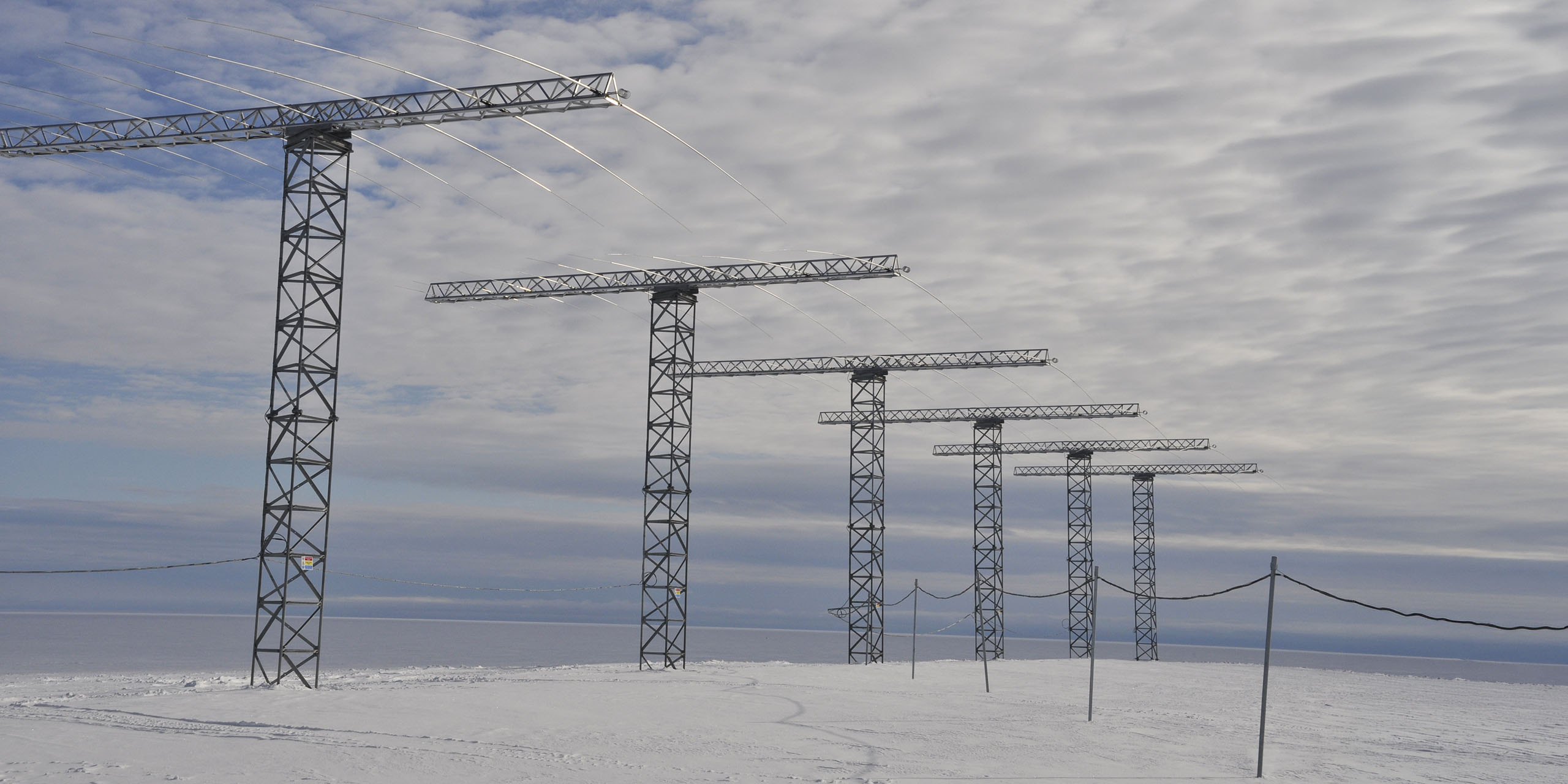
| Data Collection: | The data from this archive were taken by the UHF (ultra-high frequency) and VHF (very-high frequency) radars, situated in Ramfjordmoen, near Tromso (detailed description in Rishbeth & Williams, 1985) The UHF consists of a fully steerable, 32 metre parabolic dish and operates at frequencies close to 930 MHz, with a peak power of 2 MW. The 3 MW VHF radar is a 40 by 120 metre parabolic trough with an elevation range of 15-90deg and an operating frequency of 224 MHz. The data were analysed using the GUISDAP 9 package, downloaded from: https://gitlab.com/eiscat/guisdap9 |
|---|
Storage
| Distribution: | |
|---|---|
| Distribution Media | Online Internet (HTTP) |
| Distribution Size | N/A |
| Distribution Format | N/A |
| Fees | N/A |
| Data Storage: | We have created be 84 different files, 20 for UHF, 20 VHF for 1 hour and 10 minute integration periods (named 'radar_year_integration.h5', e.g. uhf_2001_10_mins.h5). These HDF5 file contains (the 2D arrays are altitude by time which may change by year): Alt - Altitude - (dimensions = n_elements(alt) x n_elements(time)) double array giving the altitude for each time step (km) Az - Azimuth - (dimension = 1 x n_elements(time)) double array containing the azimuth angle of the radar (degrees) Coll - Collision Frequency - (dimensions = n_elements(alt) x n_elements(time)) - double array containing the collision frequency (s-1) Coll_err - Error in the Collision Frequency - (dimensions = n_elements(alt) x n_elements(time)) -double array containing the errors associated with the collision frequency (s-1) Comp - Composition - ion species content: ion mix [O2+,NO+]/N, oxygen ions [O+]/N - (dimensions = n_elements(alt) x n_elements(time)) El - Elevation - (dimension = 1 x n_elements(time)) double array containing the elevation angle of the radar (degrees) Magic Const - Magic Constant - (dimension = 1 x n_elements(time)) string array containing the calibration scale factor Name_Expr - Experiment/Pulse Code Name - (dimension = 1 x n_elements(time)) string array. Ne - Electron Density - (dimensions = n_elements(alt) x n_elements(time)) - double array containing the electron density measurement for each step in altitude and time (m-3) Ne_err - Error in the electron density -(dimensions = n_elements(alt) x n_elements(time)) -double array giving the errors for each electron density measurement (m-3) Pt - "Peak Power of Transmitter" - (dimension = 1 x n_elements(time)) double array giving the power of the transmission (W) Range - (dimensions = n_elements(alt) x n_elements(time)) double array giving the range of the antenna measurements (m) Te - Electron Temperature - (dimensions = n_elements(alt) x n_elements(time)) -double array containing the electron temperature measurement each step in altitude and time (K) Te_err - Error in the electron temperature - (dimensions = n_elements(alt) x n_elements(time)) -double array giving the errors for each electron temperature measurement (K) Ti - Ion Temperature - (dimensions = n_elements(alt) x n_elements(time)) -double array containing the ion temperature measurement each step in altitude and time (K) Ti_err - Error in the Ion temperature - (dimensions = alt x time) -double array giving the errors for each ion temperature measurement (K) Time1 - (dimension = 1 x n_elements(time))) double array containing the start time for the integration period for each measurement (s) Time2 - (dimension = 1 x n_elements(time)) double array containing the end time for the integration period for each measurement (s) Tsys - System Temperature - (dimension = 1 x n_elements(time))) double array (K) Vi - Ion Velocity - (dimensions = n_elements(alt) x n_elements(time)) - double array containing the ion velocity measurement each step in altitude and time (ms-1) Vi_err - Error in the ion velocity - (dimensions = n_elements(alt) x n_elements(time)) - double array giving the errors for each ion velocity measurement (ms-1) We have also created 84 power profile H5 files (named radar_year_integration_pp.h5, e.g. uhf_2001_1_hour_pp.h5) containing: Alt_pp - double array containing the altitude steps of the raw power profile data (dimension = time by alt) in m. pp -"Raw_Electron_Density", double array (dimensions n_elements(alt) x n_elements(time)) pp_err - "Error_in_Raw_Electron_Density", double array (dimensions n_elements(alt) x n_elements(time)) time1_pp - "Start_Time_of_Integration_Period_Unix_Time", double array (dimensions 1 x n_elements(time)) time2_pp - "End_Time_of_Integration_Period_Unix_Time", double array (dimensions 1 x n_elements(time)) |